Wikipedia is a rich source of information and knowledge. Conveniently structured into articles with categories and links to other articles, it also forms a network of related documents. My NLP project downloads, processes, and applies machine learning algorithms on Wikipedia articles.
In my last article, KMeans clustering was applied to a set of about 300 Wikipedia articles. Without any expected labels, the clustering result could only be approached by checking which articles were grouped together and which word most frequently appeared. The results were not convincing, e.g. articles about artificial intelligence were grouped together with articles about space exploration.
To improve clustering results, this article approaches three different goals. First, visualize the document vectorization results and draw the clusters. Second, apply different vectorization methods. Third, use additional clustering algorithms.
The technical context of this article is Python v3.11 and scikit-learn v1.2.2. All examples should work with newer library versions too.
Context
This article is part of a blog series about NLP with Python. In my previous articles, I covered how to use the WikipediaReader object to download 100 subpages from the articles “Machine Learning”, “Spacecraft”, and “Python (programming language)”, creating a corpus of about 300 articles. The articles, mere text files, are further processed by an WikipediaCorpus object for summarizing the totality of all articles. A Pandas DataFrame object is then created containing the title, text, preprocessed text, and the tokens for each article. Finally, the preprocessed text is vectorized and used as input to a clustering algorithm.
Goal 1: Visualization
The first goal is to better understand the vector space of documents. In the article series so far, a bag-of-word dictionary was converted to a vector with the SciKit Learn built-in DictVectorizer. Following code snippet shows its application and gives an impression about the resulting vectors:
from sklearn.feature_extraction import DictVectorizer

vectorizer = DictVectorizer(sparse=False)
x_train = vectorizer.fit_transform(X['bow'])

print(type(x_train))
#numpy.ndarray

print(x_train)
#[[ 15.   0.  10. ...   0.   0.   0.]
# [662.   0. 430. ...   0.   0.   0.]
# [316.   0. 143. ...   0.   0.   0.]
# ...
# [319.   0. 217. ...   0.   0.   0.]
# [158.   0. 147. ...   0.   0.   0.]
# [328.   0. 279. ...   0.   0.   0.]]

print(x_train.shape)
# (272, 52743)

print(vectorizer.get_feature_names_out())
# array([',', ',1', '.', ..., 'zy', 'zygomaticus', 'zygote'], dtype=object)

print(len(vectorizer.get_feature_names_out()))
# 52743
As you can see, the resulting vectors have 52743 dimensions.
For drawing them, we will apply dimensionality reduction with PCA, and then plot it. Applying 2D PCA on the training data, and then drawing a plot, is achieved with the following code:
import matplotlib.pyplot as plt
from sklearn.decomposition import PCA

def pca_reduce(vec_list, dimensions=2):
    return PCA(dimensions).fit_transform(vec_list)

def d2_plot(data):
    plt.plot(data, 'o')

d2_plot(pca_reduce(x_train,2))
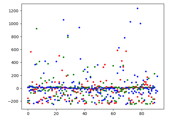
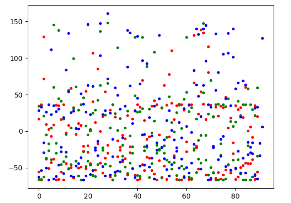
There is no clear separation in the data points, they are more or less centered around the y-axis with a zero value, and some outliers. Will this graph change when another dimensionality reduction mechanism is used?
The following code applies TruncatedSVD to the data.
import matplotlib.pyplot as plt
from sklearn.decomposition import TruncatedSVD

def pca_reduce(vec_list, dimensions=2):
    return TruncatedSVD(dimensions, n_iter=40).fit_transform(vec_list)

def d2_plot(data):
    plt.plot(data, '.')

d2_plot(pca_reduce(x_train,2))
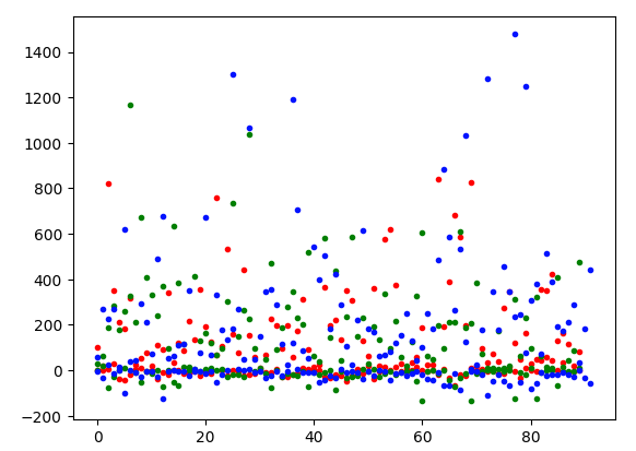
The graph looks a bit different, less outliers on the y-axis with values smaller than 0.
Finally, lets view the data as a 3D graph.
import matplotlib.pyplot as plt
from sklearn.decomposition import PCA

def pca_reduce(vec_list, dimensions):
    return PCA(dimensions).fit_transform(vec_list)

def d3_plot(data):
    fig = plt.figure()
    ax = fig.add_subplot(projection='3d')
    for _, v in enumerate(data[:90]):
        ax.scatter(v[0],v[1], v[2],marker='.', color='r')
    for _, v in enumerate(data[90:180]):
        ax.scatter(v[0],v[1], v[2],marker='.', color='g')
    for _, v in enumerate(data[180:]):
        ax.scatter(v[0],v[1], v[2],marker ='.', color='b')

    plt.show()

d3_plot(pca_reduce(x_train,3))
In this graph too, the data points are very closely related.
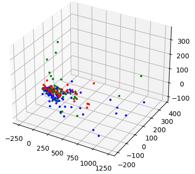
These visualizations show one clear liability of using a bag-of-word document representation: The resulting vectors are close to each other, making it difficult for a clustering algorithm to separate the documents properly. To better differentiate the data, we need to use another vectorization method and visually compare the resulting vector space.
Goal 2: Apply different Vectorization Methods
Following the assumption that changing the vectorization method can lead to better separated vectors and therefore to a better clustering, this section presents two different vectorization methods: Tfidf and WordVectors.
Tfidf Vectorization
SciKit Learn has a built-in Tfidf Vector which can be applied to raw text data. During setup of this project, a special preprocessed representation of the raw data was produced, in which all words are represented as their lemmas, and most stop words removed. The Tfidf vector will be computed on this data.
Here is the relevant code:
from sklearn.feature_extraction.text import TfidfVectorizer

x_train = X['preprocessed'].tolist()

vectorizer = TfidfVectorizer()
x_train = vectorizer.fit_transform(x_train)

print(x_train.shape)
# (272, 40337)

print(x_train)
# (0, 1002) 0.010974360184074128
# (0, 5031) 0.011294684416460914
# (0, 30935) 0.013841666362619034
# (0, 1004) 0.010228010133798603
# (0, 22718) 0.009819505656781956
# (0, 1176) 0.012488241517746365
# (0, 4398) 0.012488241517746365
# (0, 8803) 0.015557383558602929
# (0, 36287) 0.028985349686940432
The resulting vector space has only 40337 dimensions. Applying both 2D and 3D PCA on the resulting vectors gives the following graphs:

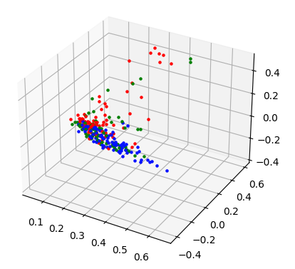
The 2D graph shows a clearer separation between the data points, and in 3D, we see some differences between the red and green marked points.
WordVector Vectorization
Word vectors represent each word with a multidimensional value that represents its meaning in the context of the trained corpus material. As covered in earlier articles, different pre-trained word vector representation exists, and the Gensim library provides them as convenient downloads.
In the following example, the Glove Gigaword pre-trained vectors with 50 dimensions are used. The DataFrame object already defines a token list derived from the preprocessed text (only lemmas, no stop words), and from it, a new column with the word vectors is created.
import gensim.downloader as api
import numpy as np

vocab = corpus.vocab()
vector_lookup = api.load('glove-wiki-gigaword-50')

word_vector(tokens):
    return np.array([
        vector_lookup[token]
        for token in tokens
        if token in vocab and token in vector_lookup
    ])

X['word_vector'] = X['tokens'].apply(lambda tokens: word_vector(tokens))
Running this code yields the following enhanced DataFrame object:
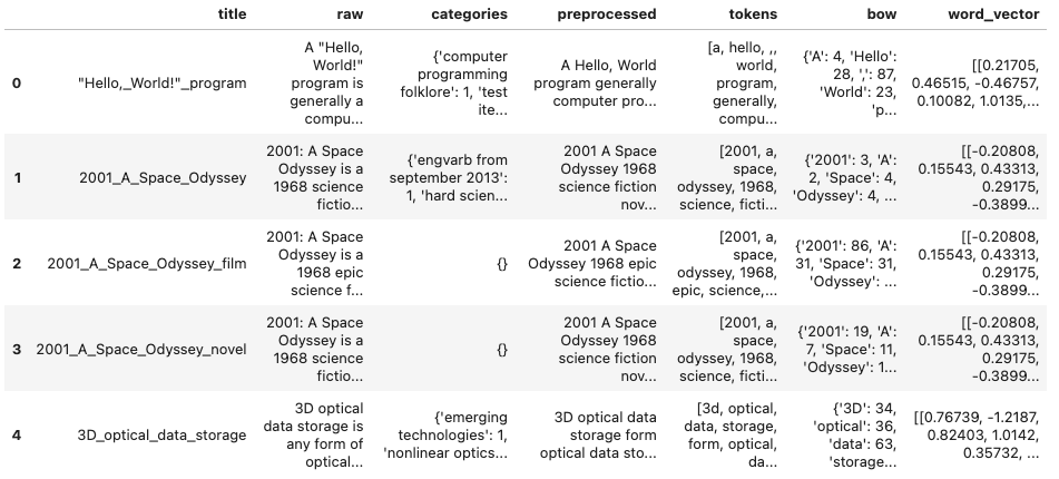
In its current form, the word vectors have different lengths. Printing their length verbose, and drawing a histogram is achieved with the following code:
word_vector_length = np.array([len(tokens) for tokens in X['word_vector'].to_numpy().flatten()])

print(word_vector_length[:5])
# [760, 157, 7566, 2543, 2086]

bins=int(np.max(word_vector_length)/1000)

plt.hist(x=word_vector_length,  bins=bins, density=False)
plt.show()

print(f'Mean: {word_vector_length.mean()}')
# Mean: 2248.904411764706
The histogram clearly shows that shorter article texts are the norm:

To apply PCA, the vectors need to padded and truncated. I choose a maximum word length of 6000, which means to pad/truncate to 300000.
def pad_word_vectors(vec_list, padding_value):
    res = []
    for vec in vec_list:
        con = np.array([v for v in vec]).reshape(-1)
        con_padded = np.pad(con, (0, padding_value))
        con_truncated = con_padded[:padding_value]
        res.append(con_truncated)
    return np.array(res)

def pca_reduce(vec_list, n_components):
    return PCA(n_components).fit_transform(vec_list)

X = pd.read_pickle('ml29_01_word_vectors.pkl')
x_train = X['word_vector'].to_numpy()

x_train_padded = pad_word_vectors(x_train,300000)

x_train_2d = pca_reduce(x_train_padded,2)
x_train_3d = pca_reduce(x_train_padded,3)
The truncated and padded vectors represented as 2D and 3D vectors:

Both graphs show a clear separation of the data points.
To summarizes: The initial DictVectorizer of a bag-of-word put the documents very close to each other. Using Tfidf and especially WordVectors clearly distributes the documents better.
Goal 3: Apply Clustering Algorithms
KMeans is only one of many clustering algorithms. Following the advice from this blog post about topic modelling, the clustering algorithm should be chosen based on how clearly separable the data is. For example, K-Means works well with low dimensional values on small datasets, and Density Based Spatial Clustering (DBSCAN) is better when the clusters have variable densities and sizes, and in general the data is high dimensional. Both of these approaches create flat cluster, while another group of algorithms creates hierarchical clusters, like Ward or the Hierachical Density Based Spatial Clustering method which is implemented by the HDBSCAN Paython library.
Based on this, I decided to use the DBSCAN and OPtics algorithm, which the documentatation refers to as better suited for large datasets. KMeans is used as the baseline.
Clustering with Tfidf Vectors
KMeans with Tfidf
When using KMeans, the expected number of clusters need to be given a-prori. Experimenting with different numbers and checking the resulting document distributions is the key.
The following code shows the result of creating 8 clusters:
model = KMeans(n_clusters=8, random_state=0, n_init="auto").fit(x_train)
print(model)
# KMeans(n_init='auto', random_state=0)

print(model.get_params())
#{'algorithm': 'lloyd', 'copy_x': True, 'init': 'k-means++', 'max_iter': 300, 'n_clusters': 8, 'n_init': 'auto', 'random_state': 0, 'tol': 0.0001, 'verbose': 0}

print(model.labels_)
#[4 6 6 6 6 4 2 4 2 4 2 4 2 2 2 2 2 2 2 2 4 4 4 4 4 4 2 4 3 4 0 6 5 6 3 2 4
# 1 4 5 4 0 1 2 1 1 2 2 0 6 2 1 2 1 5 5 2 2 7 2 5 5 5 5 5 4 4 2 4 1 2 2 2 2
# 5 2 2 2 4 0 5 5 2 6 6 2 5 0 0 5 0 1 4 4 2 5 0 2 2 2 6 6 4 6 0 0 5 2 2 4 4
# 0 0 5 1 1 1 1 6 2 0 2 2 5 4 2 4 4 4 1 2 1 2 2 2 0 4 4 4 4 2 4 3 6 3 3 7 7
# 3 3 1 2 2 2 2 4 4 1 1 4 4 2 2 2 0 2 2 4 6 6 2 4 0 0 7 6 4 6 7 2 4 6 6 1 7
# 4 1 1 1 4 7 4 4 4 4 4 6 5 7 4 4 7 2 6 4 5 6 6 6 6 6 3 4 5 1 1 5 3 3 5 1 6
# 3 3 6 1 6 6 1 1 6 6 6 6 3 3 2 3 1 3 1 3 3 6 1 6 5 6 5 3 6 6 1 3 3 3 3 5 6
# 5 6 6 3 7 2 3 2 1 4 6 3 1]
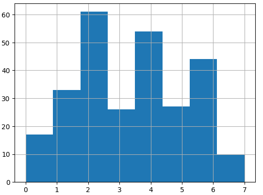
The visual representation shows un-equal separation of the clusters:
Let’s try to create 5 clusters.
model = KMeans(n_clusters=8, random_state=0, n_init="auto").fit(x_train)

print(model.labels_)
# [0 2 2 2 4 0 2 0 4 3 3 4 3 3 3 3 3 3 3 3 0 0 0 0 0 4 3 4 4 4 3 4 2 4 4 3 4
#  4 0 2 3 0 1 3 4 2 4 3 0 4 3 1 3 2 2 2 3 3 0 3 2 2 2 4 4 4 0 3 0 2 3 3 3 3
#  1 3 3 3 4 3 1 4 3 2 2 3 2 0 0 2 0 1 4 4 3 2 0 3 2 2 2 2 0 2 2 0 1 3 2 4 0
#  0 3 4 1 1 1 1 2 3 3 3 3 4 0 3 4 0 0 1 3 1 3 3 3 3 0 0 0 0 3 0 4 2 4 4 0 0
#  4 4 4 3 3 3 3 4 0 1 1 4 0 3 3 3 3 3 3 4 1 2 3 4 0 3 0 4 4 2 0 3 0 2 1 1 0
#  4 1 1 2 4 0 0 0 0 0 0 2 2 0 0 0 0 4 4 4 2 2 2 2 1 2 4 0 2 1 1 2 4 4 4 1 2
#  4 4 2 2 2 2 2 1 4 2 2 2 4 4 3 4 1 4 1 4 4 2 2 2 2 2 2 4 4 2 2 4 4 4 4 2 2
#  2 2 2 4 0 3 4 3 2 0 4 2 1]
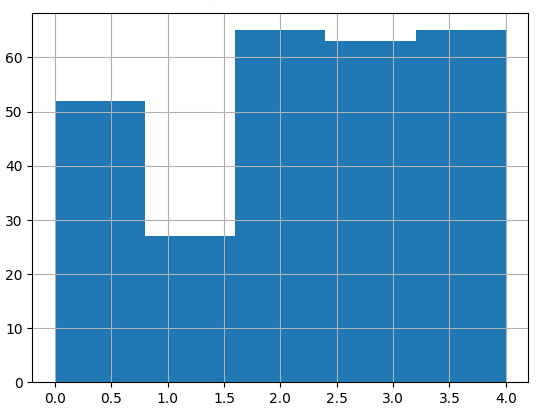
The histogram for 5 clusters shows a clear separation:
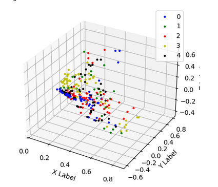
Drawing the documents in a 3D graph is also very promising:
DBSCAN with Tfidf
The following code snippet loads the pickles data, extracts the preprocessed text, and applies the Tfidf vectorizer. Then, the DBSCAN algorithm is created by instantiating the SciKit learn object.
from sklearn.feature_extraction.text import TfidfVectorizer
from sklearn.cluster import DBSCAN
import pandas as pd

X = pd.read_pickle('ml29_01.pkl')
x_train = X['preprocessed'].tolist()

vectorizer = TfidfVectorizer()
x_train = vectorizer.fit_transform(x_train)
Using DBSCAN without any parametrization gives a very surprising result:
model = DBSCAN()
print(model.get_params())
# {'algorithm': 'auto', 'eps': 0.5, 'leaf_size': 30, 'metric': 'euclidean', 'metric_params': None, 'min_samples': 5, 'n_jobs': None, 'p': None}


print(model.labels_)
# [-1 -1 -1 -1 -1 -1 -1 -1 -1 -1 -1 -1 -1 -1 -1 -1 -1 -1 -1 -1 -1 -1 -1 -1
# -1 -1 -1 -1 -1 -1 -1 -1 -1 -1 -1 -1 -1 -1 -1 -1 -1 -1 -1 -1 -1 -1 -1 -1
# ...
#  -1 -1 -1 -1 -1 -1 -1 -1]
The value -1 means that the data is too noisy and could not be clustered. What is the reason for this? Is it because Tfidf vectors are sparse? This can be remedied with TruncatedSVD.
from sklearn.decomposition import TruncatedSVD

def pca_reduce(vec_list, n_components):
    return TruncatedSVD(n_components).fit_transform(vec_list)

x_train_3d = pca_reduce(x_train, 3)

model = DBSCAN().fit(x_train_3d)

print(model.get_params())
# {'algorithm': 'auto', 'eps': 0.5, 'leaf_size': 30, 'metric': 'euclidean', 'metric_params': None, 'min_samples': 5, 'n_jobs': None, 'p': None}

print(model.labels_)
# [0 0 0 0 0 0 0 0 0 0 0 0 0 0 0 0 0 0 0 0 0 0 0 0 0 0 0 0 0 0 0 0 0 0 0 0 0
# 0 0 0 0 0 0 0 0 0 0 0 0 0 0 0 0 0 0 0 0 0 0 0 0 0 0 0 0 0 0 0 0 0 0 0 0 0
# ...
# 0 0 0 0 0 0 0 0 0 0 0 0 0]
Now, all documents are put into the one and only vector.
OPTICS with Tfidf
The optics algorithm could not run on the matrix type sparse that’s returned by the TfODF vectorizer. It needs to be converted to a dense matric beforehand by applying a Numpy conversion methods.
from sklearn.feature_extraction.text import TfidfVectorizer
from sklearn.cluster import OPTICS

X = pd.read_pickle('ml29_01.pkl')
x_train = X['preprocessed'].tolist()

vectorizer = TfidfVectorizer()
x_train = vectorizer.fit_transform(x_train).todense()
Applying the OPTICS algorithm with one parameter gives the following results:
model = OPTICS(min_samples=10).fit(np.array(x_train))

print(model.get_params())
#{'algorithm': 'auto', 'cluster_method': 'xi', 'eps': None, 'leaf_size': 30, 'max_eps': inf, 'memory': None, 'metric': 'minkowski', 'metric_params': None, 'min_cluster_size': None, 'min_samples': 10, 'n_jobs': None, 'p': 2, 'predecessor_correction': True, 'xi': 0.05}

print(model.labels_)
#[0 0 0 0 0 0 0 0 0 0 0 0 0 0 0 0 0 0 0 0 0 0 0 0 0 0 0 0 0 0 0 0 0 0 0 0 0
# 0 0 0 0 0 0 0 0 0 0 0 0 0 0 0 0 0 0 0 0 0 0 0 0 0 0 0 0 0 0 0 0 0 0 0 0 0
# ...
# 0 0 0 0 0 0 0 0 0 0 0 0 0]
Unfortunately, all documents are put into one, and only one, cluster again.
Summary of using Tfidf
Using Tfidf vectors showed only good results for KMeans clustering. Especially with 5 clusters, a clear separation could be achieved. DBSCAN and Optics instead only place all documents in the same cluster.
Clustering with WordVectors
KMeans with Word Vectors
Applying Word Vectors follows the same process as described above, loading their representation from the DataFrame, then apply padding and truncation to 300.000 values (6000 words).
This time, KMeans showed a surprise: When using the 300.000 length vectors, all documents are put into one cluster as well:
x_train_padded = pad_word_vectors(x_train,300000)

n_clusters = 5
model = KMeans(n_clusters, random_state=0, n_init="auto").fit(x_train_padded )

print(model.labels_)
# [2 2 2 2 2 2 2 2 2 2 2 2 2 2 2 2 2 2 2 2 2 2 2 2 2 2 2 2 2 2 2 2 2 2 2 2 2
#  2 2 2 2 2 2 2 2 2 2 2 2 2 2 2 2 2 2 2 2 2 2 2 2 2 2 2 2 2 2 2 2 2 2 2 2 2
#  2 2 2 2 2 2 2 2 2 2 2 2 2 2 2 2 2 2 2 2 2 2 3 2 2 2 2 2 2 2 2 2 2 2 2 2 2
#  2 2 2 2 2 2 2 2 2 2 2 2 2 2 2 2 2 2 2 2 2 2 2 2 2 2 2 2 2 2 2 2 4 2 2 2 2
#  2 2 2 2 2 2 2 2 2 2 2 2 2 2 2 2 2 2 2 2 2 2 2 2 0 2 2 2 2 2 2 2 2 2 2 2 2
#  2 2 2 2 2 2 2 2 2 2 2 2 2 2 2 2 2 2 2 2 2 2 2 2 2 2 2 2 2 2 2 2 2 2 2 2 2
#  2 2 2 2 2 2 2 2 2 2 2 2 2 2 2 2 2 2 2 2 2 2 1 2 2 2 2 2 2 2 2 2 2 2 2 2 2
#  2 2 2 2 2 2 2 2 2 2 2 2 2]
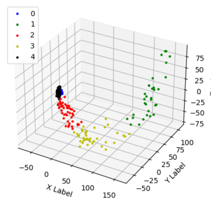
Reducing them to 3D vectors creates a good separation:
x_train_padded = pad_word_vectors(x_train,300000)
x_train_3d = pca_reduce(x_train_padded,3)

n_clusters = 5
model = KMeans(n_clusters, random_state=0, n_init="auto").fit(x_train_3d)

print(model.labels_)
#[0 0 1 2 2 2 2 0 0 0 0 4 0 3 0 4 0 2 4 3 4 4 1 0 3 4 0 3 4 0 0 0 4 4 4 4 0
# 4 2 0 0 0 3 2 4 4 2 3 0 4 0 3 0 3 1 2 0 0 0 0 4 0 0 1 4 2 1 1 2 1 0 0 0 0
# 0 2 2 4 0 4 0 0 2 2 3 4 4 4 0 0 0 0 2 2 4 2 1 4 1 2 2 2 3 4 1 3 0 0 3 0 4
# 4 0 0 2 1 4 2 1 4 0 0 3 0 4 2 2 2 4 1 0 0 1 4 3 0 2 3 4 4 0 4 4 2 0 2 0 0
# 4 3 1 0 0 4 0 4 2 1 2 2 3 0 0 0 4 0 0 3 0 2 0 3 0 0 0 3 0 0 0 3 0 2 4 2 0
# 3 0 0 2 4 0 3 1 0 0 4 4 3 0 0 1 0 3 4 4 1 2 0 1 0 4 3 3 2 4 0 1 1 0 0 1 3
# 3 2 3 2 4 0 4 1 4 4 0 0 4 4 4 2 4 0 0 2 2 3 1 1 2 1 1 0 0 4 1 3 4 3 3 1 2
# 1 3 3 0 3 3 4 4 4 2 0 4 1]
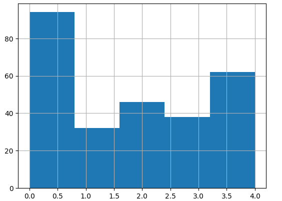
Here is the histogram and the 3D representation for all clusters:
Additionally, lets see the WordClouds for the cluster 1 and 5. As can
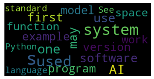
As can be seen, cluster 1 is about Python, software, system and model.

And the cluster 5 is about spacecraft, satellite, and space. This distinguishing looks promising to me.
DBSCAN
Let’s see how DBSCAN processes the new cluster data.
x_train_padded = pad_word_vectors(x_train,300000)

model = DBSCAN().fit(x_train_3d)

print(model.labels_)
# [-1  0 -1 -1 -1 -1 -1  0 -1 -1  0 -1 -1 -1 -1 -1 -1 -1 -1 -1 -1 -1 -1 -1
#  -1 -1 -1 -1 -1 -1  0 -1 -1 -1 -1 -1 -1 -1 -1 -1  0 -1 -1 -1 -1 -1 -1 -1
#   0 -1 -1 -1  0 -1 -1 -1 -1  0  0 -1 -1  0  0 -1 -1 -1 -1 -1 -1 -1  0 -1
#  -1 -1 -1 -1 -1 -1 -1 -1 -1 -1 -1 -1 -1 -1 -1 -1 -1 -1 -1 -1 -1 -1 -1 -1
#  -1 -1 -1 -1 -1 -1 -1 -1 -1 -1 -1  0 -1 -1 -1 -1 -1 -1 -1 -1 -1 -1 -1 -1
#   0 -1 -1 -1 -1 -1 -1 -1 -1 -1 -1 -1 -1 -1 -1 -1 -1 -1 -1 -1 -1 -1 -1 -1
#  -1 -1 -1  0 -1 -1 -1 -1 -1 -1 -1 -1 -1 -1 -1 -1 -1 -1  0  0 -1  0 -1 -1
#  -1 -1 -1 -1 -1  0  0 -1  0 -1 -1 -1 -1 -1 -1 -1  0 -1 -1 -1 -1 -1 -1 -1
#  -1 -1 -1 -1 -1 -1  0 -1 -1 -1 -1 -1 -1 -1 -1 -1 -1 -1 -1 -1 -1 -1 -1 -1
#  -1 -1 -1 -1 -1 -1 -1 -1 -1 -1 -1 -1 -1 -1 -1 -1 -1 -1 -1 -1 -1 -1 -1 -1
#  -1 -1 -1 -1 -1 -1 -1 -1 -1  0 -1 -1 -1 -1 -1 -1 -1 -1 -1 -1 -1 -1 -1 -1
#  -1 -1 -1 -1 -1 -1 -1 -1]
Unfortunately, using 300.000 dimensions puts all results into 1 cluster. And with the 3D PCA reduced vectors, several documents remain detected as -1, too noisy data.
To improve the DBSCAN results, I tried different parameters, like DBSCAN(eps=1.0, min_samples=10, algorithm='brute', but to no avail - the clustering results remained. Another option is to define a custom distance function, but I did not apply it in the scope of this article.
Optics
The OPTICS algorithm shows the same results when using the 300.000 dimensional vectors:
x_train_padded = pad_word_vectors(x_train,300000)

model = OPTICS(min_samples=10).fit(np.array(x_train_padded))

print(model.labels_)
# [-1  0 -1 -1 -1 -1 -1  0  0 -1  0 -1 -1 -1  0 -1 -1 -1 -1 -1 -1 -1 -1 -1
#  -1 -1 -1 -1 -1 -1  0 -1 -1 -1 -1 -1 -1 -1 -1 -1  0  0 -1 -1 -1 -1 -1 -1
#   0 -1 -1 -1  0 -1 -1 -1  0  0  0 -1 -1  0  0 -1 -1 -1 -1 -1 -1 -1  0 -1
#   0 -1  0 -1 -1 -1 -1 -1  0 -1 -1 -1 -1 -1 -1 -1  0 -1  0  0 -1 -1 -1 -1
#  -1 -1 -1 -1 -1 -1 -1 -1 -1 -1 -1  0 -1 -1 -1 -1 -1 -1 -1 -1 -1 -1 -1 -1
#   0 -1 -1 -1 -1 -1 -1 -1 -1 -1 -1 -1 -1 -1 -1 -1 -1 -1 -1 -1 -1 -1 -1 -1
#  -1 -1 -1  0 -1 -1 -1 -1  0 -1 -1 -1 -1 -1 -1 -1 -1 -1  0  0 -1  0  0 -1
#  -1 -1 -1 -1 -1  0  0 -1  0 -1 -1 -1 -1 -1 -1 -1  0 -1  0 -1 -1 -1 -1 -1
#  -1 -1 -1 -1 -1 -1  0 -1 -1 -1 -1 -1 -1 -1 -1 -1 -1 -1 -1 -1 -1 -1 -1  0
#  -1 -1 -1 -1 -1 -1 -1 -1 -1 -1 -1  0 -1 -1 -1 -1 -1 -1 -1 -1 -1 -1 -1 -1
#  -1 -1 -1 -1 -1 -1 -1 -1 -1  0  0 -1 -1 -1 -1 -1 -1 -1 -1 -1 -1 -1 -1 -1
#  -1 -1 -1 -1 -1  0 -1 -1]
But when plotting the 3D version, clusters start to emerge.
x_train_3d = pca_reduce(x_train_padded,3)

model = OPTICS(min_samples=10).fit(np.array(x_train_3d))

print(model.labels_)
# [-1  2  5 -1 -1 -1 -1  2  2  0  2  3 -1 -1  1  3 -1 -1  4 -1  4  3  5 -1
#  -1  3  0 -1  4  1  2  0 -1  4 -1 -1 -1  4 -1 -1  2  2 -1 -1 -1 -1 -1 -1
#   2 -1  1 -1  2 -1  5 -1  2  2  2  1  4  2  2  5  4 -1  5  5 -1  5  2  0
#   2  0  2 -1 -1  3  0 -1  2  1 -1 -1 -1  3  3 -1  2  0  2  2 -1 -1  4 -1
#   5 -1  5 -1 -1 -1 -1  3 -1 -1  1  2 -1 -1  3  3 -1  1 -1  5  4 -1  5  3
#   2 -1 -1  0 -1 -1 -1 -1 -1  5 -1  1  5  4 -1  1 -1 -1  4  4  1  4 -1 -1
#  -1 -1 -1  2  3 -1  5  1  1  4  0 -1 -1  5 -1 -1 -1  0  2  2 -1  2  2 -1
#  -1 -1 -1 -1  0  2  2 -1  2  1 -1 -1  1 -1 -1 -1  2 -1  2  1 -1  4  0 -1
#   5 -1  1  3  3 -1  2  1  5 -1 -1  4 -1 -1 -1  1  5 -1 -1 -1 -1 -1 -1  2
#  -1  5 -1  1  5 -1 -1 -1 -1 -1 -1  2 -1  5  4 -1 -1  1  3 -1  4 -1 -1  1
#  -1 -1 -1 -1  5  5 -1  5  5  2  2 -1  5 -1 -1 -1 -1 -1 -1 -1 -1 -1  0 -1
#  -1 -1 -1 -1 -1  2 -1 -1]
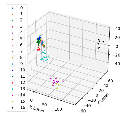
After some parameter tweaking, I finally arrived at the following representation:
model = OPTICS(min_samples=5, metric='minkowski').fit(np.array(x_train_3d))

print(model.get_params())
# {'algorithm': 'auto', 'cluster_method': 'xi', 'eps': None, 'leaf_size': 30, 'max_eps': inf, 'memory': None, 'metric': 'minkowski', 'metric_params': None, 'min_cluster_size': None, 'min_samples': 5, 'n_jobs': None, 'p': 2, 'predecessor_correction': True, 'xi': 0.05}

print(model.labels_)
# [-1 -1 18 -1 -1 12 -1 -1  3 -1  4  8  6 15 -1  9  6 -1 10 -1 10  8 -1 -1
#  -1  8  0 16 10 -1  4  0 11 10  9 11 -1 10 13 -1  5 -1 15 13 11  9 14 -1
#   5  9 -1 15 -1 -1 -1 -1  3  5 -1 -1 10 -1 -1 18 10 -1 -1 -1 -1 -1 -1  0
#  -1  0  2 14 -1  7  0 10  3 -1 14 13 -1  8 -1  9  5  0  3  3 -1 -1 10 -1
#  -1 11 -1 -1 13 -1 15 -1 -1 16 -1  4 16 -1 -1 -1 -1 -1 -1 18 10 13 18  7
#   4 -1 17 -1 11 -1 -1 12 11 -1 -1  1 -1 10 -1 -1 12 17 10 10 -1 10  9 -1
#   6 12 -1 -1  7 -1 18  1 -1 11  0 -1 -1 -1 -1 14 15  0  4  4 11  5  3 -1
#  -1 -1  6 16 -1  4  4 -1 -1 -1 -1 16  1 13 -1 13  5 17  2  1 13 10  0 -1
#  -1 -1  1  7  8 -1  5 -1 -1 -1 15 10  9 19 13 -1 -1 -1  9 -1 -1 13  9  2
#  19 18  6 -1 -1 15 17 12 -1 13  9  2 11 -1 10 11  6 -1  8  9 10 -1  9 -1
#   7 14 12 -1 18 -1 13 18 19  4  2 -1 18 15 11 17 15 19 -1 19 -1 -1  0 -1
#  15 11 10 11 14  3 11 -1]
The histogram and the 3D plotting show that the clusters are separated:

Summary of using WordVectors
WordVectors produced surprising results. In general, using 300.000 dimensional original vectors is not applicable: The variance of the data, determined by the word order of each text, is to big to find meaningful cluster. A dimensionality reduction technique needs to be applied. And then again, KMeans showed the best separation, followed by OPTICS.
Conclusion
Document classification results are dependent on the shape of the input data as well as the classification algorithm. Following a rather disappointing result when using simple bag-of-word vectors with KMeans, this article combined Tfidf and Word Vectors with KMeans, DBSCAN and Optics. The most crucial learning points from these experiments are this: a) Tfidf provides a clean separation that can be used without dimensionality reduction, b) WordVectors can only be applied after dimensionality reductions, c) KMeans provides good clustering results without any need of parametrization, d) OPTICS provides good clusters as well, but its parameters need to be tuned.
